HSP90¶

1. Introduction¶

Accurately sampling binding-site hydration can be a limiting factor in relative binding free energy (RBFE) calculations. Buried water molecules can exchange with bulk on timescales that are much slower than typical RBFE, and their slow rearrangement can lead to hysteresis, poor overlap between alchemical states.

To address this, this tutorial demonstrates hybrid MD/MC water sampling, using either (i) Grand Canonical Monte Carlo (GCMC) water insertion/deletion or (ii) a Water Swap Monte Carlo (Water MC) scheme that shift water molecules between the active site and the bulk.

In this tutorial we use the HSP90 Woodhead dataset from Schrödinger. The protein–ligand input structures are adapted from Ross et al. [1], which highlighted that explicit water sampling using GCMC can substantially improve sampling efficiency for this system. We reproduce that setting here and provide two water-enhanced sampling modes implemented in this package:

GCMC: water molecules are inserted into or deleted from a predefined region (typically the binding site) while the simulation box and the number of non-water particles remain fixed. Conceptually, the binding site is coupled to an water reservoir at a specified chemical potential.
Water MC: a pairwise move is attempted where one water is deleted from the active-site region and another is inserted in the bulk (or the reverse). This enforces constant total water count while accelerating the exchange of waters between the active site and bulk. The simulation is performed in the NPT ensemble.

2. Preparation¶

2.1. Environment setup¶

#!/usr/bin/env bash
mamba activate grandfep_dev
export script_dir="/GrandFEP_Gitdir/Script/"

GrandFEP_Gitdir should be replaced by your GrandFEP git repository directory. The scripts under Script/ will be used throughout the tutorial.

2.2. Ligand preparation¶

# from the GrandFEP root directory
cd test/hspw_tutorial/lig_prep

All of the ligands have been prepared by Antechamber. 02.mol2 has the AM1-BCC charges and 03.frcmod has the missing parameters. The Amber tleap script 04_tip3p_150mmol.in, and the solvated water box 03_all_ligands_solvated.pdb are also provided.

./04_build_box.sh

After running 04_build_box.sh, Amber top (.prmtop) and coordinate (.inpcrd) file will be generated in each ligand folder. Those files are : 07_tip3p.pdb, 07_tip3p.prmtop,07_tip3p.inpcrd for tip3p water and 08_opc.pdb, 08_opc.prmtop, 08_opc.inpcrd for OPC water.

2.3. Protein preparation¶

# from the GrandFEP root directory
cd test/hspw_tutorial/pro_prep

Files are provided.

2.4. Check atom mapping¶

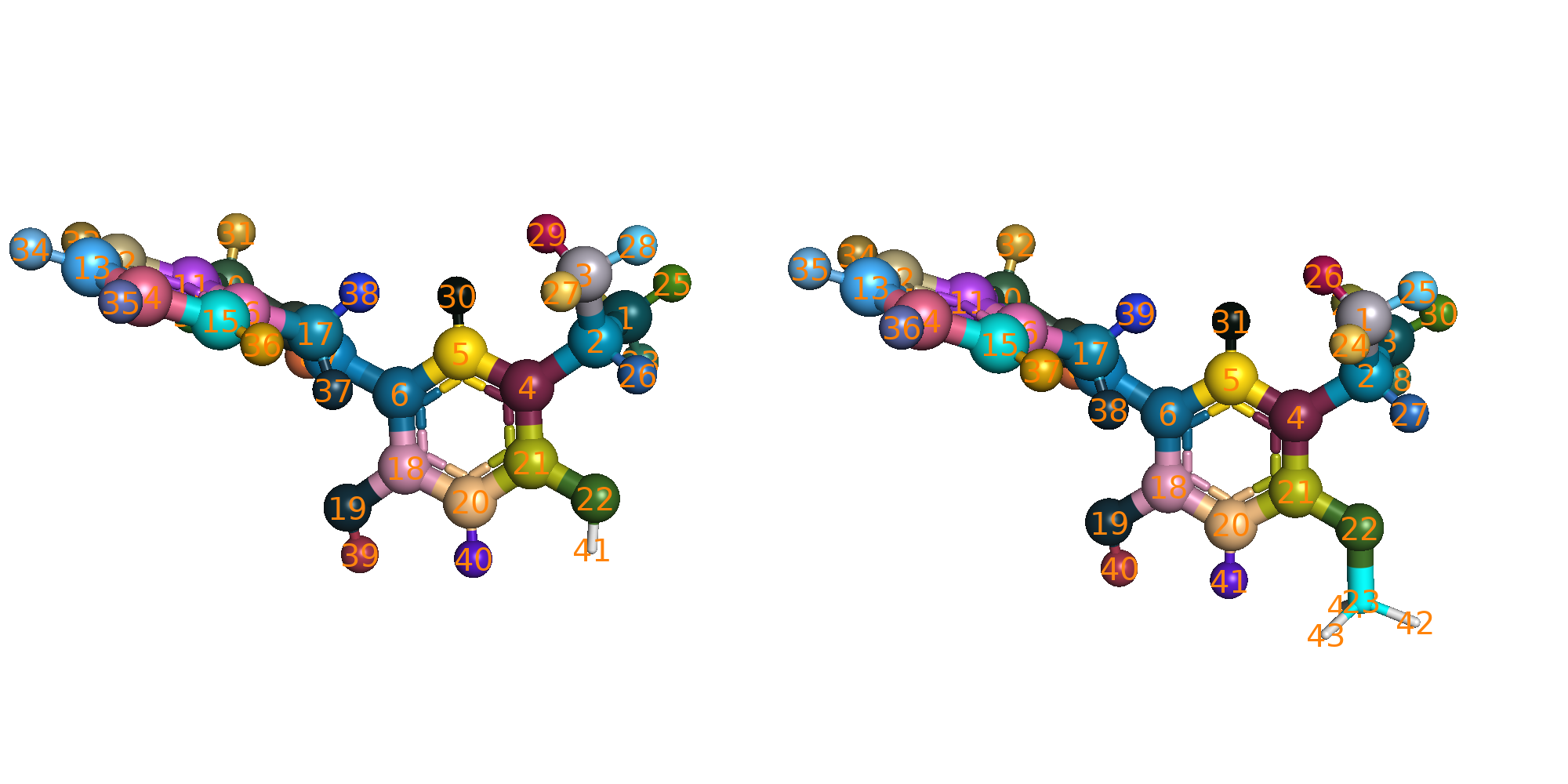
The atom mapping is provided in each edge (edge_LigX_to_LigY) folder. You can visualize the mapping by excuting the following script.

# from the GrandFEP root directory
cd JOB/atom_mapping/
./run_check_all.sh

The pymol script $script_dir/color_map_pairs.py will be called to load and color the mapped atoms. Mapped atoms will have the same color showing in sphere.
mapping

2.5. Hybrid system preparation¶

# from the GrandFEP root directory
cd test/hspw_tutorial/JOB/tip3p_REST2
./run_01_hybrid.sh

This will take a while. This script prepares the hybrid topologies (the system object in openmm), and save the system to a serialized file system.xml.gz. This can save time in the later simulations. Here is a quick explanation of the script for doing this hybrid system preparation.

$script_dir/hybrid.py \
    -prmtopA A.prmtop \
    -inpcrdA A.inpcrd \
    -prmtopB B.prmtop \
    -inpcrdB B.inpcrd \
    -yml ../hybrid_map.yml \
    -pdb system.pdb \
    -system system.xml.gz \
    -REST2 \
    -dum_dihe_scale 0.0 1.0 0.0 0.0 0.0

prmtop and inpcrd are the Amber topology and coordinate files.
yml is the yaml file that contains the atom mapping and nonbonded settings. An example is given below.
system.pdb is the output pdb file for saving the hybrid topology (openmm.topology has atom, bond and residue information).
system.xml.gz is the compressed serialized hybrid system file.
-REST2 use REST2. Dihedral and nonbonded terms of the selected REST2 atoms will be scaled.
-dum_dihe_scale scales the dummy dihedral terms in the hybrid system. Here we set the scaling factors for dummy dihedrals with periodicity 1, 2, 3, 4, 5 to be 0.0 1.0 0.0 0.0 0.0, meaning only the periodicity 2 dummy dihedrals are kept. This can give flexibility to the dummy atoms but stop double bond from isomerization.

yaml example:

mapping_list:
- index_map:
    0: 2
    1: 1
    2: 0
    3: 3
  res_nameA: MOL
  res_nameB: MOL
# map res MOL in state A to res MOL in state B with the above atom index mapping

# nonbonded settings for HMR (hydrogen mass repartitioning). They will be passed to AmberPrmtopFile.createSystem()
system_setting:
  nonbondedMethod: "app.PME"
  nonbondedCutoff: "1.0 * unit.nanometer"
  constraints    : "app.HBonds"
  hydrogenMass   : "3.0 * unit.amu"

2.6. Center selection¶

# from the GrandFEP root directory
cd test/hspw_tutorial/JOB/tip3p_REST2/protein/center_selection
pymol run_check.py

There are 2 types of GC moves: GC_sphere and GC_box. GC_sphere tries to insert/delete water molecules within a sphere centered at a specified atom. GC_box tries to insert/delete water molecules in the whole simulation box. GC_sphere actively samples water molecules in the binding site, while GC_box generates density fluctuations. GC_sphere needs a center atom to define the sphere. We check this center selection here. The selected center atom will be shown in sphere.

Please change the 2nd C19 atom in edge_3_to_2/tip3p_REST2/protein/system.pdb to something else (e.g., C99)

< HETATM41019  C19 MOL B   1      38.771  38.915  39.837  1.00  0.00           C  
---
> HETATM41019  C99 MOL B   1      38.771  38.915  39.837  1.00  0.00           C 

3. Water leg NPT¶

3.1. Preparation¶

Only one edge will be demonstrated.

# from the GrandFEP root directory
cd test/hspw_tutorial/edge_1_to_2/tip3p_REST2/
cat ../OPT_lam.yml

An optimized lambda schedule for 16 window FEP is provided in OPT_lam.yml. We will use this lambda schedule to run the water leg NPT simulations.

# window Indices                            0,             1,             2,             3,
lambda_angles               : [ 0.000000, 0.066667, 0.133333, 0.200000,] # ... linear
lambda_bonds                : [ 0.000000, 0.066667, 0.133333, 0.200000,] # ... linear
lambda_sterics_core         : [ 0.000000, 0.066667, 0.133333, 0.200000,] # ... linear
lambda_electrostatics_core  : [ 0.000000, 0.066667, 0.133333, 0.200000,] # ... linear
lambda_torsions             : [ 0.000000, 0.066667, 0.133333, 0.200000,] # ... linear
k_rest2                     : [ 1.000000, 0.904286, 0.808571, 0.712857,] # 1.0 ~ 0.33 ~ 1.0
#
# lambda_total                  0.00000000000, 0.03895141349, 0.08555498164, 0.14334167206, 
# = lambda_electrostatics_delete + lambda_sterics_delete + lambda_electrostatics_insert
lambda_electrostatics_delete: [ 0.000000, 0.116854, 0.256665, 0.430025,]
# lambda_sterics_delete = lambda_sterics_insert
lambda_sterics_delete       : [ 0.000000, 0.000000, 0.000000, 0.000000,]
lambda_sterics_insert       : [ 0.000000, 0.000000, 0.000000, 0.000000,]
lambda_electrostatics_insert: [ 0.000000, 0.000000, 0.000000, 0.000000,]

lambda_angles, lambda_bonds, lambda_torsions, lambda_sterics_core, lambda_electrostatics_core are linearly spaced from 0 to 1. k_rest2 scales down the interaction of REST2 (hot) atoms. The interaction is scaled down to 0.33 at the middle windows (window 7 and 8), which is effectivly increasing the temperature to 298.15K / 0.33 = 903.5K.

These 4 lambda values are optimized (non-linear)

lambda_electrostatics_delete turns off the charges on atoms that exist in state A but become dummy atoms in state B.
lambda_sterics_delete turns off the vdW interaction on atoms that exist in state A but become dummy atoms in state B.
lambda_sterics_insert turns on the vdW interaction on atoms that exist in state B but stay dummy in state A.
lambda_electrostatics_insert turns on the charges on atoms that exist in state B but stay dummy in state A.

lambda_sterics_delete and lambda_sterics_insert are set with the same values, and the total process is defined as lambda_electrostatics_delete + lambda_sterics_delete + lambda_electrostatics_insert. This gives us a 1-dimensional path optimization problem. The lambda schedule optimization is not covered in this tutorial.

We are going to prepare the simulation parameter yaml files here:

# from the GrandFEP root directory
cd test/hspw_tutorial/edge_1_to_2/tip3p_REST2/
mkdir -p water/NPT/
cp ../../JOB/tip3p_REST2/water/NPT/rep_999 ./water/NPT/ -r

cd water/NPT/rep_999/

sed 's/GEN_VEL/true/'  npt_tmp.yml > ./npt_eq.yml
sed 's/GEN_VEL/false/' npt_tmp.yml > ./npt.yml

for win in {0..15}
do
    mkdir $win -p
    sed "s/INIT_LAMBDA_STATE/$win/" npt_eq.yml > $win/npt_eq.yml
    sed "s/INIT_LAMBDA_STATE/$win/" npt.yml    > $win/npt.yml
    cat ../../../OPT_lam.yml >> $win/npt_eq.yml
    cat ../../../OPT_lam.yml >> $win/npt.yml
done
cd ../

These yaml files contain the simulation parameters for each window.

3.2. Equilibration¶

Run the following script to equilibrate each window individually.

# from the GrandFEP root directory
cd test/hspw_tutorial/edge_1_to_2/tip3p_REST2/water/NPT/
cp rep_999/ rep_0/ -r
cd rep_0/
base=$PWD
batch_size=4 # 16 windows in batch of 4, you can do batch of 8 if you have more CPUs
for win0 in $(seq 0 $batch_size 15)
do
    win1=$((win0+batch_size-1))
    for win in $(seq $win0 $win1)
    do
        cd $base/$win
        if [ ! -f npt_eq.pdb ]; then
            echo "Run $win"
            $script_dir/run_NPT_init.py \
                -pdb ../../../system.pdb \
                -system ../../../system.xml.gz \
                -nstep 50000 \
                -yml npt_eq.yml \
                -deffnm npt_eq &
                # 50000 * 0.004 ps = 200 ps
        fi
    done
    wait
done

This will run 200 ps NPT equilibration for each window. After equilibration, you can check the csv file for temperature and density.

3.3. Production¶

Run the following script to perform production NPT simulations.

for win in {0..15}
do
    mkdir $win/0 -p
done

mpirun -np 16 $script_dir/run_NPT_RE.py \
    -pdb    ../../system.pdb \
    -system ../../system.xml.gz \
    -multidir 0 1 2 3 4 5 6 7 8 9 10 11 12 13 14 15 \
    -yml npt.yml \
    -maxh 4 \
    -ncycle 10000 \
    -start_rst7 npt_eq.rst7 \
    -deffnm 0/npt 

After 4 hour time out, if the number of RE cycles has not reached 10000, you can execute the same command again to continue the simulation. The -deffnm flag will tells the script to append the new data to existing files. The simulation will end when the number of RE reaches ncycle (10000 here).

If you want to start a new simulation in the next directory (e.g., 1/npt), you can run:

for win in {0..15}
do
    mkdir $win/1 -p
done

mpirun -np 16 $script_dir/run_NPT_RE.py \
    -pdb    ../../system.pdb \
    -system ../../system.xml.gz \
    -multidir 0 1 2 3 4 5 6 7 8 9 10 11 12 13 14 15 \
    -yml npt.yml \
    -maxh 4 \
    -ncycle 10000 \
    -start_rst7 0/npt.rst7 \
    -deffnm 1/npt

5 ~ 10 ns is sufficient.

4. NPT density equilibration¶

GC has slower density fluctuation autocorrelation time than normal NPT MD. NPT is still the better way to equilibrate the density. We run a short NPT simulation to equilibrate the density before running GC simulations. We run the same thing as the water leg ($script_dir/run_NPT_init.py).

# from the GrandFEP root directory
# Preparation
cd test/hspw_tutorial/edge_1_to_2/tip3p_REST2/protein
mkdir NPT
cp ../../../JOB/tip3p_REST2/protein/NPT/rep_999 ./NPT/ -r

cd ./NPT/rep_999/

sed 's/GEN_VEL/true/'  npt_tmp.yml > ./npt_eq.yml
sed 's/GEN_VEL/false/' npt_tmp.yml > ./npt.yml

for win in {0..15}
do
    mkdir $win -p
    sed "s/INIT_LAMBDA_STATE/$win/" npt_eq.yml >  $win/npt_eq.yml
    sed "s/INIT_LAMBDA_STATE/$win/" npt.yml    >  $win/npt.yml
    cat ../../../OPT_lam.yml                   >> $win/npt_eq.yml
    cat ../../../OPT_lam.yml                   >> $win/npt.yml
done
cd ../

# Equilibration
base=$PWD
for rep in {0..2}
do
    cd $base
    cp rep_999/ rep_$rep/ -r
    cd $base/rep_$rep/
    batch_size=4 # 16 windows in batch of 4, you can do batch of 8 or 16 if you have more CPUs
    for win0 in $(seq 0 $batch_size 15)
    do
        win1=$((win0+batch_size-1))
        for win in $(seq $win0 $win1)
        do
            cd $base/rep_$rep/$win
            if [ ! -f npt_eq.pdb ]; then
                echo "Run rep_$rep $win"
                $script_dir/run_NPT_init.py \
                    -pdb ../../../system.pdb \
                    -system ../../../system.xml.gz \
                    -nstep 100000 \
                    -yml npt_eq.yml \
                    -deffnm npt_eq &
                    # 100000 * 0.004 ps = 400 ps
            fi
        done
        wait
    done
done

The NPT RE production run can be run in the same way as the water leg.

5. GCMC¶

GC (µVT) can be relatively expensive than normal NPT, if you want to achieve the same density fluctuations. Modern simulation engines do NPT by calculating the virial and scaling the box, but GCMC (µVT) needs insertion/deletion Monte Carlo moves to generate density fluctuations and sample waters. Although the primary goal of GC is to sample water molecules in the binding site, we still need some density fluctuations.

We will run a equilibration with more GC moves in the subdir 0 in each window folder, and continue to run further simulations with less GC moves in 1, 2, 3 … subdirs ~1ns each.

5.1. Preparation of parameter files¶

Prepare the yaml files for GC simulations. We use the optimized lambda schedule from water leg NPT simulations.

# from the GrandFEP root directory
cd test/hspw_tutorial/edge_1_to_2/tip3p_REST2/protein
mkdir GC_80l_40MD_15RE_200MD
cp ../../../JOB/tip3p_REST2/protein/GC_80l_40MD_15RE_200MD/rep_999 ./GC_80l_40MD_15RE_200MD/ -r
cd GC_80l_40MD_15RE_200MD/rep_999/
# sed keyword GEN_VEL and RESTRAINT
center="C18" # each edge has its own center atom
sed -e 's/GEN_VEL/true/' \
    -e "s/RESTRAINT/false/" \
    gc_tmp.yml            >  ./gc_eq.yml
cat prot_eq.yml           >> ./gc_eq.yml
cat ../../../OPT_lam.yml  >> ./gc_eq.yml
sed -e "s/CENTERATOM/$center/" \
    GC_center.yml         >> ./gc_eq.yml

sed -e 's/GEN_VEL/false/' \
    -e "s/RESTRAINT/false/" \
    gc_tmp.yml            >  ./gc.yml
cat prot.yml              >> ./gc.yml
cat ../../../OPT_lam.yml  >> ./gc.yml
sed -e "s/CENTERATOM/$center/" \
    GC_center.yml         >> ./gc.yml

for win in {0..15}
do
    mkdir $win -p
    sed "s/INIT_LAMBDA_STATE/$win/" gc_eq.yml > $win/gc_eq.yml
    sed "s/INIT_LAMBDA_STATE/$win/" gc.yml    > $win/gc.yml
done

5.2. Preparation of starting structures¶

After the NPT equilibration, we cut a slightly smaller box on the final frame of NPT simulation. The volume that has been cut will be converted to ghost waters in the following GC simulations.

cd test/hspw_tutorial/edge_1_to_2/tip3p_REST2/protein/GC_80l_40MD_15RE_200MD
base=$PWD
for rep in {0..2}
do
    cd $base/
    cp rep_999 rep_$rep -r
    cd rep_$rep
    for win in {0..15}
    do
        cd $base/rep_$rep/$win
        # if link npt_eq.rst7 not exists, create link
        if [ ! -L npt_eq.rst7 ]; then
            ln -s ../../../NPT/rep_$rep/$win/npt_eq.rst7
        fi
    done
done
cd $base
$script_dir/run_GC_prep_box.py \
    -pdb ../system.pdb \
    -system ../system.xml.gz \
    -multidir rep_?/?/ rep_?/??/ \
    -yml gc_eq.yml \
    -start_rst7 npt_eq.rst7 \
    -odeffnm gc_start \
    -scale_box 0.996

The box will be scaled from the mean box size by 0.996. The scaled box size will be saved to gc_start.dat.

Each frame still needs to be optimized (Energy minimization). The Volume that has been cut will be converted to ghost waters. The ghost waters will be randomly chosen.

We run energy minimization on those new starting structures.

cd test/hspw_tutorial/edge_1_to_2/tip3p_REST2/protein/GC_80l_40MD_15RE_200MD
$script_dir/run_GC_prep_box.py \
    -pdb ../../system.pdb \
    -system ../../system.xml.gz \
    -multidir rep_?/?/ rep_?/??/ \
    -yml gc_eq.yml \
    -start_rst7 npt_eq.rst7 \
    -odeffnm gc_start \
    -box $(< ../gc_start.dat)

gc_start.rst7 and gc_start.jsonl will be generated in each window folder. These files will be the starting configuration for the GC simulations.

5.3. Equilibration¶

cd test/hspw_tutorial/edge_1_to_2/tip3p_REST2/protein/GC_80l_40MD_15RE_200MD/rep_0
for win in {0..15}
do
    mkdir $win/0
done
mpirun -np 16 $script_dir/run_GC_RE.py \
    -pdb    ../../../system.pdb \
    -system ../../../system.xml.gz \
    -multidir 0 1 2 3 4 5 6 7 8 9 10 11 12 13 14 15 \
    -yml gc_eq.yml \
    -maxh 18 \
    -ncycle 576 \
    -start_rst7   gc_start.rst7 \
    -start_jsonl  gc_start.jsonl \
    -deffnm       0/gc
# run until 576 RE are reached

5.4. Production¶

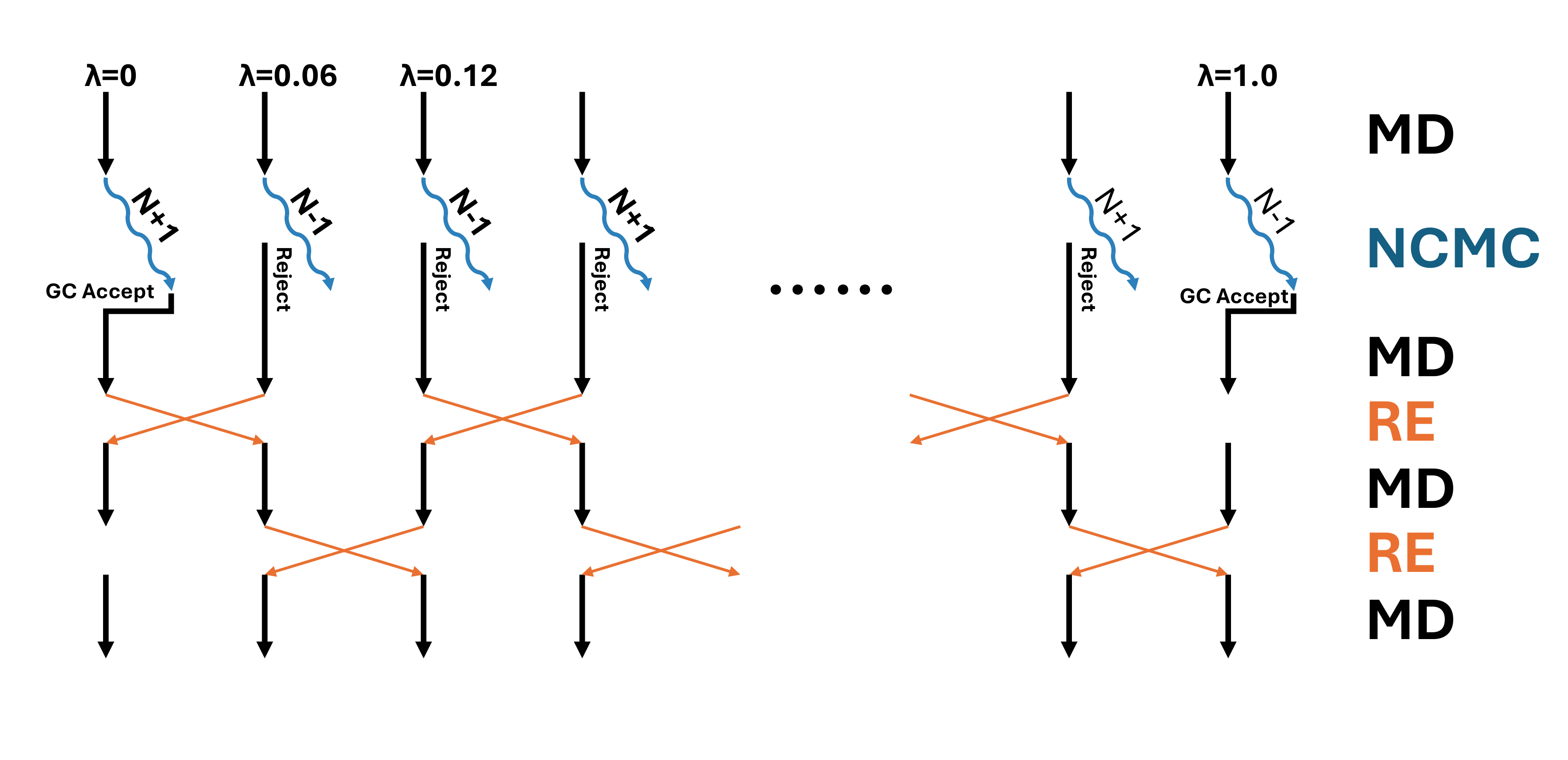Protocol In the production run, we will perform 1 GC step and 15 RE step in each sampling cycle. Between every GCor RE, 200 steps of MD will be performed. So in total, each cycle contains (1 + 15) * 200 * 0.004 = 12.8 (ps) of MD. Each 20% of the GC step is tested in the active site sphere, and the other 80% is tested in the whole box. The GC insertion/deletion Monte Carlo moves are performed in non-equilibrium fashion, with 80 perturbation steps and 40 propagation steps. In total, each GC step consists of 80 * 40 * 0.004 = 12.8 (ps) of MD.

cd test/hspw_tutorial/edge_1_to_2/tip3p_REST2/protein/GC_80l_40MD_15RE_200MD/rep_0
# run simulation in subdir 1 restarting from subdir 0
for win in {0..15}
do
    mkdir $win/1
done
mpirun -np 16 $script_dir/run_GC_RE.py \
    -pdb    ../../../system.pdb \
    -system ../../../system.xml.gz \
    -multidir 0 1 2 3 4 5 6 7 8 9 10 11 12 13 14 15 \
    -yml gc.yml \
    -maxh 9 \
    -ncycle 1200 \
    -start_rst7  0/gc.rst7 \
    -start_jsonl 0/gc.jsonl \
    -deffnm      1/gc
# run until 1200 RE are reached

Roughly 5 ns * 3 replica or 15 ns * 1 replica are needed.

5.5. MBAR¶

Estimate free energy differences (ddG in this case) with MBAR.

cd test/hspw_tutorial/edge_1_to_2/tip3p_REST2/protein/GC_80l_40MD_15RE_200MD/rep_0

partN=10 # subdirs 1-10 in each window folder should be finished
tempdir=$(mktemp -d -p /tmp rep_${rep}_part${partN}_mbar_XXXXXX)

echo "rep_$rep part $partN MBAR ..."
mkdir -p mbar_${partN}ns
cd       mbar_${partN}ns
for i in $(seq 1 $partN)
do
    mkdir -p $tempdir/0/$i
    cp ../0/$i/gc.log $tempdir/0/$i/
done
for win in {0..15}
do
    grep "T   =" $tempdir/0/1/gc.log | tail -n 1  >  $tempdir/$win.dat
    for i in $(seq 1 $partN)
    do
        grep " - INFO: $win:" $tempdir/0/$i/gc.log  >> $tempdir/$win.dat
    done
    sed -i "s/- INFO: $win:/Reduced_E:/" $tempdir/$win.dat
    awk 'NR % 3 == 1' $tempdir/$win.dat > ./$win.dat # only use 1/3 data for MBAR to save time, they are highly correlated anyway
done
rm -r $tempdir/*
$script_dir/analysis/MBAR.py -log ?.dat ??.dat -kw "Reduced_E:" -m MBAR -csv mbar_dG.csv > mbar.log 2> mbar.err
rm ?.dat ??.dat
rm -r $tempdir

The log file mbar.log will contain the ddG estimation results. The values are in kcal/mol.

Calculating free energy using MBAR method.
 A - B :   MBAR                    
----------------------------------
- 1 :  10.4122 +-  0.0137 0.40
- 2 :  10.1342 +-  0.0160 0.23
- 3 :   9.5982 +-  0.0245 0.16
- 4 :   8.5886 +-  0.0291 0.24
- 5 :   7.5752 +-  0.0220 0.26
- 6 :   7.0142 +-  0.0155 0.21
- 7 :   8.6529 +-  0.0161 0.19
- 8 :   0.8920 +-  0.0136 0.24
- 9 :  -7.0965 +-  0.0170 0.22
-10 :  -6.8383 +-  0.0187 0.17
-11 :  -6.4083 +-  0.0254 0.21
-12 :  -5.7017 +-  0.0209 0.24
-13 :  -5.8165 +-  0.0156 0.28
-14 :  -6.1015 +-  0.0183 0.12
-15 :  -6.3838 +-  0.0232 0.22
----------------------------------
Total  :  18.5210 +-  0.1064  

Three replicas results I got are:

>>> tail rep_?/mbar_10ns/mbar.log -n 1
==> rep_0/mbar_10ns/mbar.log <==
Total  :  18.5210 +-  0.1064     

==> rep_1/mbar_10ns/mbar.log <==
Total  :  19.3289 +-  0.0924     

==> rep_2/mbar_10ns/mbar.log <==
Total  :  19.1379 +-  0.1013 

We can subtract the ddG on the water leg.

\[ \Delta G_{protein} - \Delta G_{water} = (19.329 + 19.138 + 18.521)/3 - (16.4323 + 16.4013 + 16.3133)/3 = 2.61 (kcal/mol) \]

The experimental ddG is 1.98 kcal/mol. +1.98 kcal/mol means that Lig1 binds stronger than Lig2. The MD result is quite close to the experimental value. Please check the analysis/dG.ipynb for error estimation.

6. Water MC¶

6.1. Preparation of parameter files¶

Prepare the yaml files for GC simulations. We use the optimized lambda schedule from water leg NPT simulations.

# from the GrandFEP root directory
cd test/hspw_tutorial/edge_1_to_2/tip3p_REST2/protein
mkdir WaterMC_80l_40MD
cp ../../../JOB/tip3p_REST2/protein/WaterMC_80l_40MD/rep_999 ./WaterMC_80l_40MD/ -r
cd WaterMC_80l_40MD/rep_999/
# sed keyword GEN_VEL and RESTRAINT
center="C18" # each edge has its own center atom
sed -e 's/GEN_VEL/true/' \
    -e 's/RESTRAINT/false/' \
    npt_tmp.yml           >  ./npt_eq.yml
cat prot_eq.yml           >> ./npt_eq.yml
cat ../../../OPT_lam.yml  >> ./npt_eq.yml
sed -e "s/CENTERATOM/$center/" \
    GC_center.yml         >> ./npt_eq.yml

sed -e 's/GEN_VEL/false/' \
    -e "s/RESTRAINT/false/" \
    npt_tmp.yml           >  ./npt.yml
cat prot.yml              >> ./npt.yml
cat ../../../OPT_lam.yml  >> ./npt.yml
sed -e "s/CENTERATOM/$center/" \
    GC_center.yml         >> ./npt.yml

for win in {0..15}
do
    mkdir $win -p
    sed "s/INIT_LAMBDA_STATE/$win/" npt_eq.yml > $win/npt_eq.yml
    sed "s/INIT_LAMBDA_STATE/$win/" npt.yml    > $win/npt.yml
done

6.2. Copy the starting structures¶

cd test/hspw_tutorial/edge_1_to_2/tip3p_REST2/protein/WaterMC_80l_40MD
base=$PWD
for rep in {0..2}
do
    cd $base/
    cp rep_999 rep_$rep -r
    cd rep_$rep
    for win in {0..15}
    do
        cd $base/rep_$rep/$win
        # if link npt_eq.rst7 not exists, create link
        if [ ! -L npt_eq.rst7 ]; then
            ln -s ../../../NPT/rep_$rep/$win/npt_eq.rst7
        fi
    done
done

6.3. Equilibration¶

cd test/hspw_tutorial/edge_1_to_2/tip3p_REST2/protein/WaterMC_80l_40MD/rep_0
for win in {0..15}
do
    mkdir $win/0
done
mpirun -np 16 $script_dir/run_NPT_waterMC_RE.py \
    -pdb    system.pdb \
    -system system.xml.gz \
    -multidir 0 1 2 3 4 5 6 7 8 9 10 11 12 13 14 15  \
    -yml npt_eq.yml \
    -maxh 15 \
    -ncycle 576 \
    -start_rst7   npt_eq.rst7 \
    -deffnm       0/npt
# run until 576 RE cycles are finished

6.4. Production¶

In the production run, we will perform 1 water MC move and 63 RE moves in each sampling cycle. Between every water MC or RE, 200 steps of MD will be performed. So in total, each cycle contains (1 + 63) * 200 * 0.004 = 51.2 (ps) of MD. The water swap Monte Carlo moves are performed in non-equilibrium fashion, with 80 perturbation steps and 40 propagation steps. In total, each MC step consists of 80 * 40 * 0.004 = 12.8 (ps) of MD.

cd test/hspw_tutorial/edge_1_to_2/tip3p_REST2/protein/WaterMC_80l_40MD/rep_0
# run simulation in subdir 1 restarting from subdir 0
for win in {0..15}
do
    mkdir $win/1
done
mpirun -np 16 $script_dir/run_NPT_waterMC_RE.py \
    -pdb    system.pdb \
    -system system.xml.gz \
    -multidir 0 1 2 3 4 5 6 7 8 9 10 11 12 13 14 15  \
    -yml npt.yml \
    -maxh 2 \
    -ncycle 1260 \
    -start_rst7  0/npt.rst7 \
    -deffnm      1/npt
# run until 1260 RE cycles are finished

Roughly 5 ns * 3 replica or 15 ns * 1 replica are needed.

7. Collect results, and estimate ΔG¶

7.1. Run all edges¶

We need to know the ddG between every ligands to estimate the ΔG. A map of edges need to be simulated. Scripts for batch running all edges are provided.

cd test/hspw_tutorial/JOB/tip3p_REST2

7.2. Cycle closure and ΔG estimation¶

Jupyter notebook for analysis is provided in analysis/ folder.
deltaG

7.3. Shift the ghost water outside the box¶

There are ghost waters flying randomly in the simulation box. To visualize the trajectory, we can shift them away. The residue index of the ghost water is saved with the dcd file as a jsonl file.

cd test/hspw_tutorial/edge_1_to_2/tip3p_REST2/protein/GC_80l_40MD_15RE_200MD/rep_0
base=$PWD
for win in {0..15}
do
    cd $base/$win
    $script_dir/remove_ghost.py -p ../../../system.pdb \
        -idcd   [1-9]/gc.dcd   10/gc.dcd \
        -ijsonl [1-9]/gc.jsonl 10/gc.jsonl \
        -oxtc   gc_01_10.xtc
done

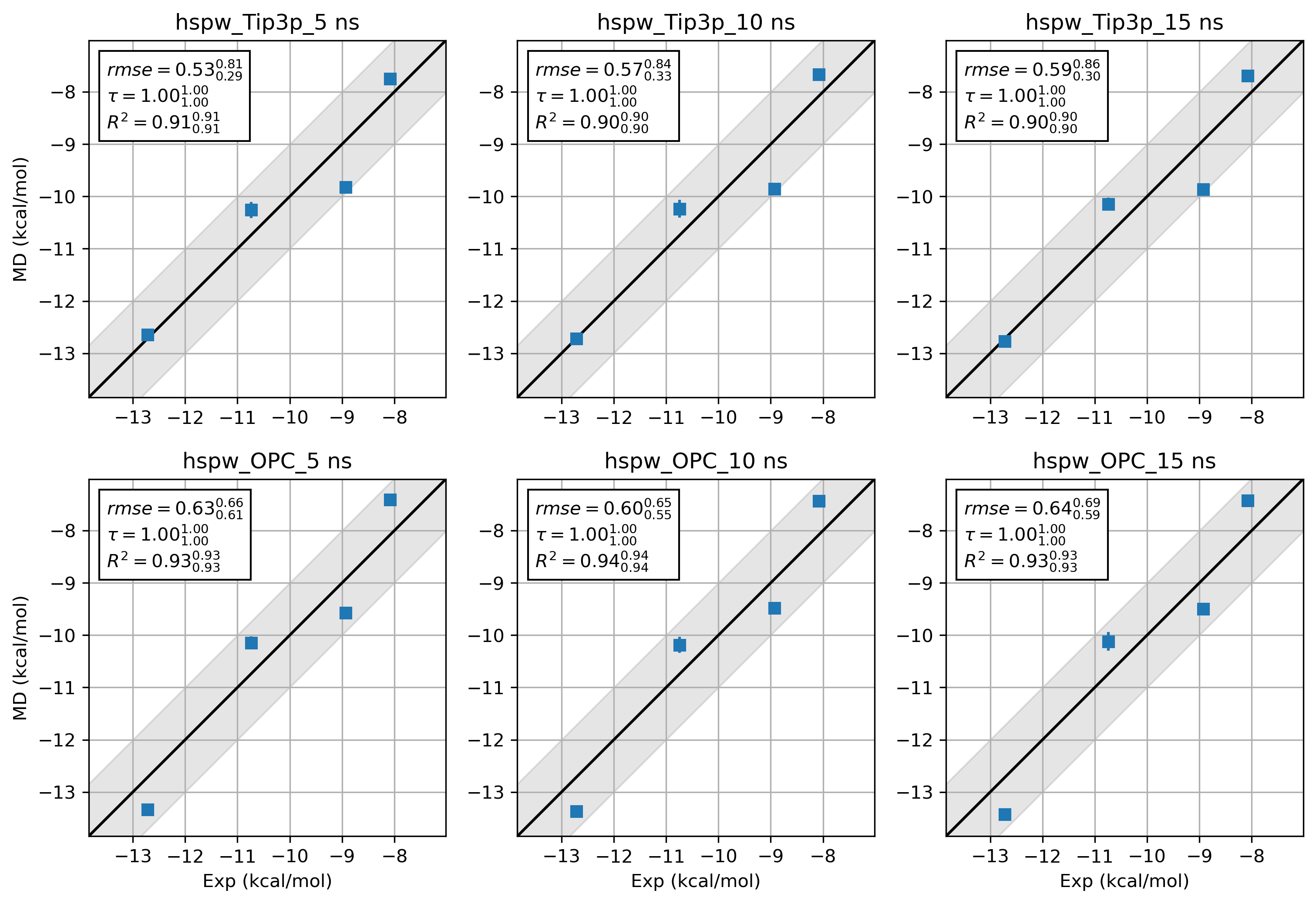
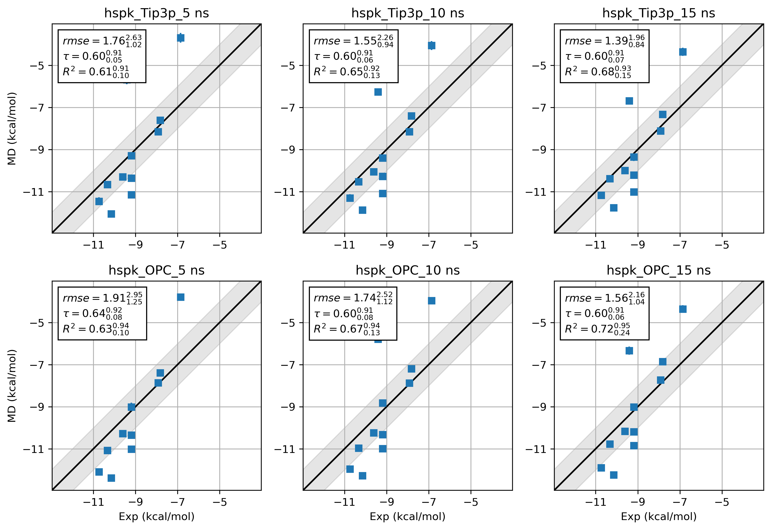
8. What about Amber19SB and OPC water?¶

It is difficult to draw a conclusion about the accuracy of 2 force field combinations. Way more benchmarks and sampling are needed. Here we just provide the results from hsp90 Kung alongside the hsp90 Woodhead data set for a quick comparison.
deltaG

9. Tips¶

9.1. How to set up the environment inside a slurm job¶

source /YourCondaInstallationDir/miniforge3/bin/activate grandfep
module add openmpi/gcc/64/4.1.5 # Remember to install the same OpenMPI version as your cluster inside the conda env

9.2. How to run OpenMPI with 2 GPUs¶

We can prepare a hostfile and an app file for mpirun.

In the case of running 16 threads on 2 GPUs (CUDA_VISIBLE_DEVICES=0,1) on a node called n71-16, the hostfile can be:

n71-16
n71-16

The app file can be:

-np 8 -x CUDA_VISIBLE_DEVICES=0 ./run_GC_RE.py -arg1 XX -arg2 XXX
-np 8 -x CUDA_VISIBLE_DEVICES=1 ./run_GC_RE.py -arg1 XX -arg2 XXX

The mpirun can be called like this:

mpirun --hostfile hostfile --app appfile

Here is a sample script for preparing appfile and hostfile for multi-GPU mpirun.

cp $script_dir/run_GC_RE.py ./
command="./run_GC_RE.py \
    -pdb system.pdb \
    -system system.xml.gz \
    -multidir 0 1 2 3 4 5 6 7 8 9 10 11 12 13 14 15 \
    -yml gc_eq.yml \
    -maxh 15 \
    -ncycle 576 \
    -start_rst7 gc_start.rst7 \
    -start_jsonl gc_start.jsonl \
    -deffnm 0/gc"

APPFILE="appfile.$SLURM_JOB_ID"
HOSTFILE="hostfile.$SLURM_JOB_ID"
> "$APPFILE"  # truncate/create
> "$HOSTFILE"

# Split CUDA_VISIBLE_DEVICES on comma into an array
IFS=',' read -ra GPU_ARRAY <<< "$CUDA_VISIBLE_DEVICES"

# if there are X GPUs, 
if [[ ${#GPU_ARRAY[@]} -eq 4 ]]; then
    for gpu in "${GPU_ARRAY[@]}"; do
        echo "$HOSTNAME" >> "$HOSTFILE"
        echo "-np 4 -x CUDA_VISIBLE_DEVICES=$gpu $command" >> "$APPFILE"
    done
elif [[ ${#GPU_ARRAY[@]} -eq 2 ]]; then
    for gpu in "${GPU_ARRAY[@]}"; do
        echo "$HOSTNAME" >> "$HOSTFILE"
        echo "-np 8 -x CUDA_VISIBLE_DEVICES=$gpu $command" >> "$APPFILE"
    done
elif [[ ${#GPU_ARRAY[@]} -eq 1 ]]; then
    for gpu in "${GPU_ARRAY[@]}"; do
        echo "$HOSTNAME" >> "$HOSTFILE"
        echo "-np 16 -x CUDA_VISIBLE_DEVICES=$gpu $command" >> "$APPFILE"
    done
else
    echo "Error: Unsupported number of GPUs (${#GPU_ARRAY[@]}). Expected 1, 2, or 4."
    exit 1
fi

echo "$(date "+%Y-%m-%d_%H:%M:%S") $HOSTFILE"
cat "$HOSTFILE"
echo "$(date "+%Y-%m-%d_%H:%M:%S") $APPFILE"
cat "$APPFILE"
echo "#########################################"

mpirun --hostfile $HOSTFILE --app $APPFILE

10. Reference¶

Ross, G. A.; Russell, E.; Deng, Y.; Lu, C.; Harder, E. D.; Abel, R.; Wang, L. Enhancing Water Sampling in Free Energy Calculations with Grand Canonical Monte Carlo. J. Chem. Theory Comput. 2020, 16 (10), 6061–6076. https://doi.org/10.1021/acs.jctc.0c00660.
XXX

11. Contact¶

Chenggong Hui (惠成功)

Email: chenggong.hui@mpinat.mpg.de
ORCID: 0000-0003-2875-4739
GitHub: GrandFEP

Here is the youtube video demonstrating this tutorial (Coming soon).

GrandFEP

Navigation

Related Topics